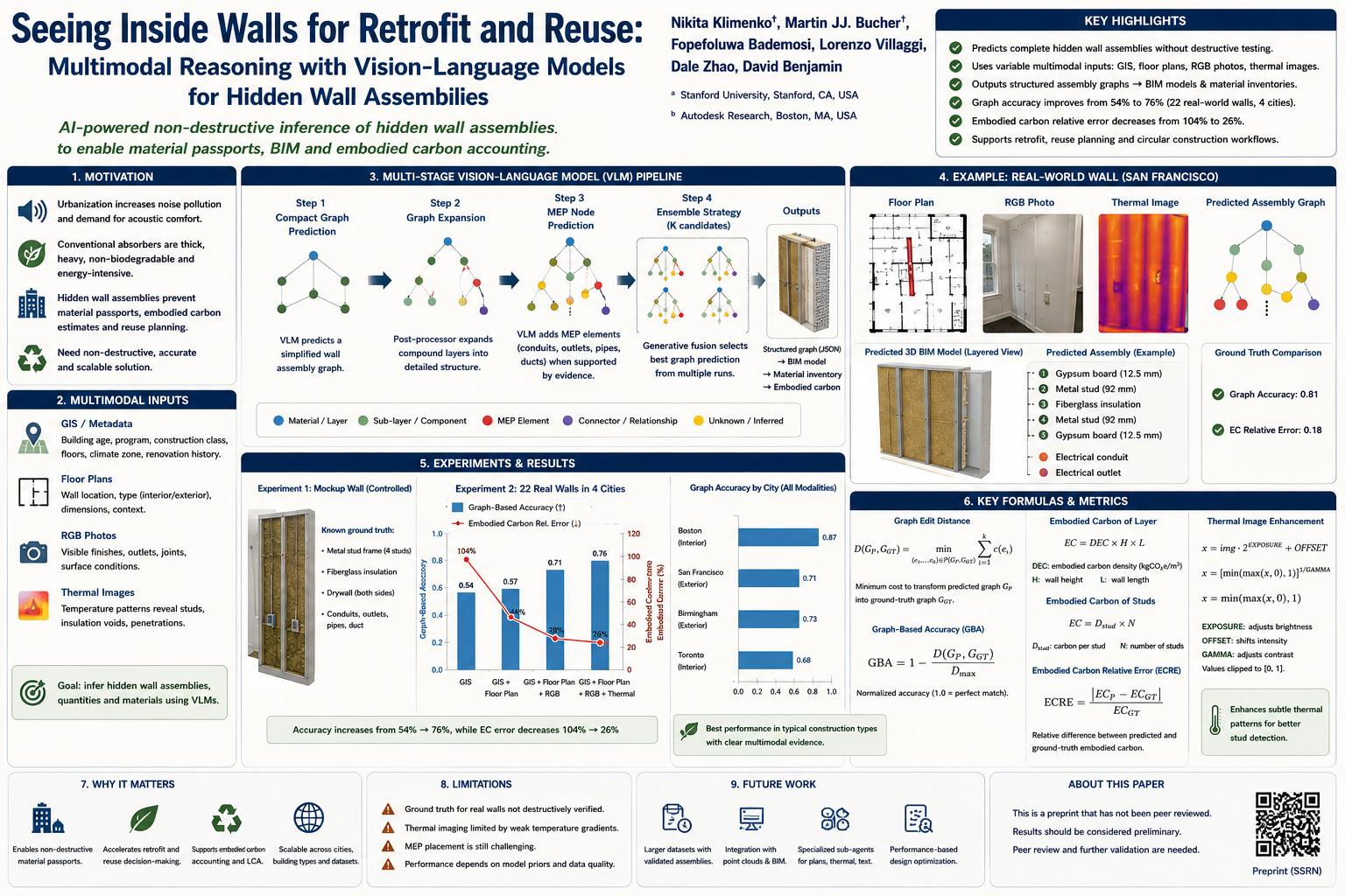
This study begins with a practical building-sector problem: existing buildings contain valuable materials, but much of that material is hidden. When a building is retrofitted, reused, renovated, or selectively demolished, designers and engineers need to know what is inside its walls. A finished wall may look simple from the outside, but internally it may contain gypsum board, studs, insulation, masonry, air gaps, conduits, pipes, outlets, membranes, or other components. These hidden layers affect reuse potential, embodied carbon, thermal performance, structural behavior, acoustic performance, fire rating, demolition cost, and material recovery.
The problem matters because retrofit and reuse are central to reducing construction-sector carbon emissions. Reusing buildings can avoid some emissions associated with new construction, but good reuse planning depends on accurate material information. If the internal wall assembly is unknown, it is hard to create a reliable material passport. It is also hard to estimate embodied carbon, plan selective deconstruction, value recoverable materials, or decide whether a wall can be retained. Traditional inspection often requires destructive testing, expert judgment, or time-consuming manual review of old drawings and BIM files. The paper asks whether AI can infer these hidden assemblies from non-destructive multimodal evidence.
The study focuses on Vision-Language Models, or VLMs. A VLM can process text and images together. Unlike a narrow machine-learning classifier trained only on one fixed dataset, a VLM has broad pretraining and can reason from different types of incomplete evidence. In this study, the model may receive GIS text, a floor plan, RGB images of the wall, and thermal images. The key idea is that no single modality is sufficient, but each modality provides a different clue. GIS data gives broad context such as building age, construction class, program, location, and climate zone. Floor plans identify whether a wall is interior or exterior and where it sits in the building. RGB photos show visible surface conditions, outlets, finishes, joints, and context. Thermal images may reveal studs or other hidden components through temperature differences.
The research gap is clear. Prior computer-vision methods can classify visible facade materials, reconstruct visible geometry, or segment building components from scans. Scan-to-BIM methods can reconstruct surfaces and objects, but they usually do not infer hidden wall layers. Thermal and RGB fusion methods can help detect defects or visible anomalies, but they do not normally generate a complete structured wall assembly. The authors therefore propose a systems-level workflow: instead of training a new model from a large labeled dataset, they carefully prompt general-purpose VLMs to infer wall assemblies and output them as structured graphs.
The workflow is summarized in Figure 1 on page 3. This figure is central to the paper. It shows the entire pipeline: multimodal input data enter the system; the VLM first predicts a compact wall graph; a non-AI post-processor expands the graph; the VLM then adds MEP nodes such as conduit and outlets; finally, an ensemble strategy compares several candidate graph predictions and selects or fuses the best prediction. The figure also shows that the output is not merely a sentence. It is a structured wall assembly graph that can be converted into a detailed assembly and later into BIM-compatible models.
The wall assembly graph is the paper’s most important representational contribution. Instead of describing a wall in plain language, the method represents it as a structured JSON object. A wall may be written as an ordered list of layers: for example, drywall, metal stud frame with fiberglass insulation, and drywall. Each layer has a material and confidence score. Compound layers, such as a stud frame, can contain nested information: number of studs and filling material. This makes the output readable by humans and processable by software.
This graph structure matters because circular construction requires machine-readable information. A narrative prediction such as “the wall probably contains metal studs and insulation” is not enough for BIM conversion or carbon accounting. A graph can be converted into a 3D model, material inventory, or embodied carbon calculation. The authors emphasize that this graph-based representation bridges VLM reasoning with downstream engineering workflows.
The method has four stages. Stage 1 predicts a compact graph. This is a simplified wall assembly, usually with three to five layers. For example, an interior partition might be predicted as drywall, metal stud frame with fiberglass insulation, and drywall. At this stage, the model must decide whether the wall is likely exterior or interior, load-bearing or non-load-bearing, masonry or stud-framed, and whether it contains insulation. One important detail is stud count: the model is asked to estimate how many studs the wall contains if a stud frame is present.
Stage 2 expands the compact graph. This is performed by a Python post-processing script rather than by the VLM. If a compact graph contains a metal stud frame with four studs and fiberglass insulation, the expansion step can turn that compound layer into individual nodes: metal channel, metal stud, insulation, metal stud, insulation, and so on. This matters because later operations may need node-level structure, not only layer-level description.
Stage 3 predicts MEP nodes. MEP means mechanical, electrical, and plumbing. In the wall context, this may include electrical conduits, outlets, pipes, or ducts. The model examines the multimodal evidence and adds these nodes only if there is strong visual or contextual evidence. This is important because MEP elements can affect reuse planning, demolition, safety, and material inventory. However, the paper also shows that MEP placement remains one of the hardest error categories.
Stage 4 uses an ensemble strategy. The same wall-and-modality combination is run multiple times because VLM outputs can vary. In the experiments, each combination is run five times independently, and the ensemble can use K = 1, 3, or 5 predictions. Instead of simple majority voting, which is hard when graph topology changes, the system uses generative fusion. The VLM reasons over several candidate graphs and produces a final prediction. This is useful because one prediction may contain an outlier, while several predictions may agree that a material is present but disagree on exact placement.
The study evaluates predictions with two main metrics: Graph-Based Accuracy and Embodied Carbon Relative Error. These formulas are important because they show how the authors measure success. The first metric checks whether the predicted wall graph structurally matches the ground-truth graph. The second checks whether the prediction is useful for embodied carbon accounting.
The first formula is the graph edit distance:
In everyday language, this formula asks: how many edits are needed to turn the predicted graph into the true graph? Here, \(G_P\) is the predicted wall graph, and \(G_{GT}\) is the ground-truth wall graph. The set \(\mathcal{P}(G_P,G_{GT})\) means all possible edit paths that could transform the predicted graph into the true one. Each edit operation \(e_i\) has a cost \(c(e_i)\). Insertions and deletions cost 1.0. A material substitution also costs 1.0, while an orientation mismatch costs 0.1. So if the model predicts drywall where the true material is concrete, that is a serious error. If it predicts the correct material but slightly wrong orientation, that is treated as a smaller error.
This formula is useful because a wall assembly is not a simple label. It is a structured object. A prediction can be partly right: it may identify drywall and insulation correctly but miss the number of studs or place an outlet incorrectly. Graph edit distance allows the evaluation to measure partial structural similarity rather than simply marking the whole prediction as right or wrong.
The second formula normalizes the edit distance and converts it into an accuracy score:
Here, GBA means Graph-Based Accuracy. \(D(G_P,G_{GT})\) is the edit distance from the first formula. \(D_{\max}\) is the maximum possible edit distance, defined using the sizes of the predicted and ground-truth trees. In simple terms, the formula turns the error distance into an accuracy value. If the predicted graph is identical to the ground truth, the distance is zero, so the accuracy becomes 1, or 100%. If the predicted graph is very different, the distance becomes larger and the accuracy falls.
The authors also handle the fact that some wall assemblies may be equivalent when reversed. A wall with drywall-stud-drywall may be read from one side or the other. Therefore, the system evaluates both the original predicted tree and a version with second-level children reversed, then reports the better match. This is sensible because the physical wall may be symmetrical or may be documented from the opposite side.
The embodied carbon calculation begins by assigning carbon values to predicted materials. For a layer such as drywall, the paper uses a formula like this:
This formula means embodied carbon equals the embodied carbon density of that material multiplied by the wall height and wall length. \(EC\) is embodied carbon. \(DEC\) is the embodied carbon density per unit area for a material layer. \(H\) is wall height, and \(L\) is wall length. In plain language, if a wall has more area, it contains more material, and therefore more embodied carbon. A default height of 10 feet is assumed for all walls.
For discrete components such as studs, the paper uses a different logic:
Here, \(D_{stud}\) is the embodied carbon per single stud, and \(N\) is the number of studs. This formula is simple but important. If the model predicts the wrong number of studs, the embodied carbon estimate changes. This is why stud count is not a minor detail. It directly affects material inventory and carbon accounting.
The third main metric is Embodied Carbon Relative Error:
This formula measures how far the predicted embodied carbon is from the ground-truth embodied carbon. \(EC_P\) is the predicted embodied carbon. \(EC_{GT}\) is the ground-truth embodied carbon. The absolute value \(|EC_P - EC_{GT}|\) means the formula cares about the size of the error, whether the prediction is too high or too low. Dividing by \(EC_{GT}\) converts the error into a relative proportion. For example, if the true embodied carbon is 100 kgCO₂e and the prediction is 126 kgCO₂e, the relative error is 26%. This metric matters because material passports and circularity assessments are not only about naming materials; they also need credible quantities and carbon estimates.
Experiment 1 uses a physical mockup wall. This is important because real hidden wall assemblies are hard to verify without destructive testing. By constructing their own wall, the authors know the exact ground truth. The mockup represents a typical partition wall in a hypothetical early-2000s Boston office building. It contains a metal stud frame with four vertical metal studs and fiberglass insulation, covered by drywall on both sides. The authors also include more complex internal elements such as conduits, outlets, pipes, and a duct.
Figure 2 on page 7 documents the mockup wall. It shows the wall assembly in progress with conduits inserted in the insulation layers, a frontal view of construction, a digital model of the wall design, a floor plan with a red bounding box showing the wall location, an RGB frontal image, and thermal images. This figure is very important because it shows the multimodal evidence given to the VLM. It also reveals a key practical issue: thermal imaging does not magically see through all wall layers. In the mockup, the duct and pipe behind insulation were mostly invisible because fiberglass insulation acted as a thermal barrier.
Table 1 on page 8 reports Experiment 1 accuracy for all combinations of data inputs and ensemble runs. The mockup experiment shows that additional modalities often improve accuracy, but not always monotonically. For example, GIS + RGB reaches 93% graph accuracy, while some combinations with more modalities produce lower accuracy. This is an important caution: more data can help, but if modalities contain conflicting or weak cues, the model may have to reconcile uncertainty and may not improve.
Still, the full combination can perform very strongly in the mockup. With GIS + floor plan + RGB + thermal data, several configurations reach 100% graph accuracy and 0% embodied carbon relative error. This does not mean the method is perfect in all real buildings. It means that under controlled conditions, with known ground truth and strong enough cues, the VLM pipeline can recover the full wall assembly graph.
Table 2 on page 8 gives example mockup predictions with graphs, 3D model outputs, and comparison to ground truth. It shows how accuracy improves as more data are added. A GIS-only prediction has low graph accuracy and very high carbon error. With more modalities, the graph becomes more complete and the embodied carbon estimate improves. This table supports the paper’s main argument that multimodal evidence can improve both structural prediction and carbon accounting.
Experiment 2 tests real-world walls. The authors collect a dataset of 22 walls across four office buildings in four cities: Boston, San Francisco, Toronto, and Birmingham. The dataset includes both interior and exterior walls. Ground truth is not obtained by destructive testing. Instead, it is established through a structured annotation protocol using existing Revit models and BIM files, architectural floor plans, renovation records, expert interpretation of thermal scans, and physical inspection by architectural professionals familiar with the buildings. This is rigorous for real-world non-destructive work, but it still contains uncertainty because the walls are not opened up.
Table 3 on page 10 gives examples from the real-world experiment. It shows floor plan inputs, RGB images, thermal images, predicted graphs, ground-truth graphs, predicted models, ground-truth models, graph-based accuracy, and embodied carbon relative error. The examples include Boston interior walls, a San Francisco exterior wall, a Birmingham exterior wall, and a Toronto interior wall. This table is one of the most informative visuals in the paper because it shows how the method performs differently across wall types and cities. Some cases improve dramatically with RGB and thermal data, while others remain difficult.
Table 4 on page 11 provides the main real-world quantitative results. Across all 22 walls, graph-based accuracy increases from 0.54 with GIS alone to 0.57 with GIS + floor plan, then to 0.71 with GIS + floor plan + RGB, and finally to 0.76 with GIS + floor plan + RGB + thermal data. This is the central performance result of the paper. It shows that each additional level of evidence generally improves prediction accuracy.
The same table shows embodied carbon relative error falling from 104% with GIS alone to 44% with GIS + floor plan, 28% with GIS + floor plan + RGB, and 26% with all modalities including thermal. This is highly important. The improvement is not only academic graph matching. Better assembly prediction translates into more accurate embodied carbon estimation. That makes the method relevant to material passports, reuse planning, and life-cycle assessment.
The location-specific results are also meaningful. Boston performs best with all modalities, reaching 0.87 graph-based accuracy and 14% embodied carbon relative error. San Francisco reaches 0.71 accuracy and 19% carbon error. Toronto reaches 0.68 accuracy and 49% carbon error. Birmingham reaches 0.73 accuracy and 30% carbon error. These differences do not necessarily mean the method works better in one city because of geography alone. The authors argue that performance differences reflect how closely each wall matches common construction patterns embedded in the model’s prior knowledge.
The paper’s discussion is careful about model priors. A VLM may infer hidden assemblies partly from evidence and partly from learned construction assumptions. For example, if it sees a modern office interior wall, it may assume drywall, metal studs, and insulation even if the evidence is weak. Sometimes this helps; sometimes it causes errors. The paper gives examples where the model misses a metal stud layer in San Francisco or incorrectly attributes stud framing to CMU-based partitions in Birmingham. This is one of the most important limitations. The model may not always “see” the wall; it may sometimes default to what similar walls usually contain.
Nevertheless, the improvement from GIS-only to full-modality input suggests that multimodal evidence contributes meaningfully beyond prior assumptions. The paper notes that accuracy improves from 47% to 74% in one comparison of model versions and from 54% to 76% in the main real-world table. Cases such as Birmingham exterior walls also show the model using visible evidence, such as brick and insulation, rather than relying only on default interior-stud assumptions.
Thermal imaging is treated as valuable but limited. It works best when there is a strong temperature differential across the wall. The appendix states that ideal stud detection requires a sustained temperature differential of at least 5–10°C, achievable through HVAC-driven gradients, solar exposure on exterior walls, or controlled heating. When the thermal gradient is weak, especially in interior partitions, thermal images show only subtle surface variations. In these cases, thermal imaging serves as a refinement rather than a dominant signal.
The study also analyzes thermal image enhancement. Equation 4 on page 14 describes an image enhancement process:
This formula adjusts a thermal image to make useful patterns easier for the model to interpret. In simple terms, \(img\) is the original image data. The exposure term brightens or darkens the image. The offset shifts the values. The gamma correction changes contrast, especially in mid-tone areas. The min-max operations clip the image so values stay between 0 and 1. The goal is not to invent information, but to make subtle thermal patterns more visible. This matters because VLMs are trained on common image patterns, and clearer stripe-like or patch-like thermal signatures may help the model identify studs.
Table 7 on page 17 reports the effect of thermal image enhancement. Without thermal data, GIS + floor plan + RGB reaches 0.71 graph-based accuracy. Adding unenhanced thermal data increases accuracy to 0.73. City-specific enhancement raises it to 0.74. Manual image-specific enhancement reaches 0.76. Embodied carbon error also reaches its best value, 26%, with image-specific enhancement. This shows that thermal preprocessing can matter, but the gains are modest. The largest improvement comes from adding RGB and other modalities, while thermal enhancement provides additional refinement.
Figure 4 on page 15 presents error analysis across 22 walls. Panel (a) shows error rate by category and modality combination. The error categories include boundary layer, structural system, stud count, stud type, MEP presence, and MEP placement. The figure shows that adding modalities reduces most error types, especially structural system and stud type identification. This makes sense because thermal and visual cues help identify framing patterns. However, MEP placement error remains difficult. The model may infer that an outlet or conduit exists, but assigning it to the exact stud bay requires fine-grained spatial reasoning that current VLMs still struggle with.
Panel (b) of Figure 4 on page 15 gives a per-wall error profile under full-modality input. It shows that errors are not evenly distributed. Exterior walls and non-standard construction types, such as CMU or mixed typologies, produce more failures than standard interior partition walls. This is an important practical caution. The method is strongest when the wall type is common and the multimodal evidence is clear. It is weaker when construction is unusual, regionally specific, poorly documented, or visually ambiguous.
Table 9 on page 18 compares two GPT model versions. GPT-5.2 reaches 0.47 graph accuracy with GIS, 0.55 with floor plan, 0.67 with RGB, and 0.74 with thermal. GPT-5.4 improves these values to 0.54, 0.57, 0.71, and 0.76. The authors interpret this as evidence that the pipeline can benefit from future foundation-model improvements without retraining. That is a meaningful systems argument: as VLMs improve, prompt-based workflows may improve too. However, it also means results depend on the model version, prompting strategy, and image preprocessing choices.
Table 10 on page 18 lists GIS metadata fields used as text input, such as year built, building program, construction class, floors, floor area, renovation history, climate zone, construction notes, and sampled walls. The table redacts identifying information. This table shows that the method does not require a perfectly standardized data package. It can use variable public-record-style data. That flexibility is valuable because real retrofit projects rarely have complete documentation.
Table 11 on page 19 gives embodied carbon coefficients and assumptions. This table is important because it shows how predicted assemblies become carbon numbers. Drywall, fiberglass insulation, concrete, CMU blocks, brick, cladding, metal studs, wooden studs, channels, conduit, and outlets are assigned kgCO₂e values per area, per stud, per linear foot, or per unit. The table also states assumptions such as 10 ft wall height, 16-inch stud spacing, and cradle-to-gate A1–A3 carbon values. These assumptions are necessary for calculation, but they also limit precision. Real walls may have different thicknesses, material products, densities, suppliers, or installation conditions.
The study’s strongest contribution is not that it perfectly identifies every hidden wall. It does not. Its strongest contribution is that it creates a practical bridge between incomplete non-destructive observations and actionable structured outputs. The workflow begins with messy data—GIS text, floor plans, photographs, thermal images—and ends with a graph that can support BIM conversion, material inventories, and carbon accounting. That is a valuable direction for circular construction.
The practical significance is considerable. If scaled, this approach could help building owners and retrofit teams create material passports for existing buildings without opening every wall. It could help estimate how much drywall, steel, insulation, brick, concrete, or CMU exists in a building. It could support selective deconstruction planning by identifying recoverable materials. It could help compare retrofit strategies based on embodied carbon and material reuse potential. It could also help prioritize walls or zones where destructive spot-checks are most needed.
However, the limitations are substantial. First, this is a non-peer-reviewed preprint, so the results have not yet been independently reviewed. Second, the real-world dataset includes only 22 walls across commercial office buildings in four cities. That is a modest dataset. It does not prove generalization to residential buildings, historic masonry, mass timber, non-Western construction systems, industrial buildings, hospitals, schools, or buildings with unusual retrofit histories.
Third, the ground truth for real walls is not destructively verified. The authors use Revit models, floor plans, renovation records, thermal scans, and expert inspection, which is reasonable and practical, but hidden assemblies can still differ from documents. Older buildings may have undocumented renovations, repairs, substitutions, or hidden damage. Therefore, the reported accuracy depends partly on the reliability of non-destructive ground-truth annotation.
Fourth, current VLMs still struggle with spatial reasoning. They may misread large floor plans, confuse thermal patterns, fail to count studs correctly, or misplace MEP elements. They also lack native point-cloud reasoning, even though point clouds are common in Scan-to-BIM workflows. Future work may need specialized sub-agents for floor plan understanding, thermal interpretation, point cloud analysis, and construction-code retrieval.
Fifth, the method may be biased toward common construction practices represented in training data. If the VLM’s pretraining contains many examples of North American office partitions, it may over-predict drywall-metal-stud-fiberglass assemblies. This can be helpful for typical buildings but risky for regional, historic, vernacular, or unconventional assemblies. The paper explicitly acknowledges this issue and calls for testing on broader typologies.
Future work proposed by the authors includes targeted spot-check verification, such as borescope inspection, to bound annotation uncertainty; semantically weighted evaluation metrics; specialized modality-specific sub-agents; larger datasets with validated assemblies; retrieval-augmented generation grounded in construction databases; extension from single-wall predictions to building-scale inventories; and performance-based generative design for reuse using predicted material inventories.
The broader meaning of the study is that AI for buildings does not need to stop at surface recognition. Existing buildings are full of hidden material information, and that information is essential for decarbonization. The paper shows a possible way to infer some of that information without demolition. It does not eliminate the need for experts, verification, or careful inspection. But it suggests that AI can help narrow uncertainty, produce structured material hypotheses, and scale building audits beyond what manual inspection alone can achieve.
For readers, the simplest interpretation is this: the study tries to help buildings “explain what is inside their walls” using the evidence already available around them. A floor plan says where the wall is. A photo says what the surface looks like. A thermal image hints at hidden framing. GIS data says what kind of building it is and when it was likely built. The VLM combines those clues and proposes a structured wall assembly. If that prediction is good enough, it can support BIM, carbon accounting, and circular reuse planning. If it is uncertain, it can guide where humans should inspect more carefully.
The work should not be read as a final replacement for building professionals or destructive verification. It should be read as an early, promising, non-peer-reviewed systems framework for non-destructive material inference. Its value lies in showing that multimodal AI can connect building documentation, hidden assembly prediction, and carbon accounting in one workflow. Its evidence level remains preliminary, but the direction is highly relevant to retrofit, reuse, and low-carbon construction.
Source and Method Note
The source analyzed here is Seeing Inside Walls for Retrofit and Reuse: Multimodal Reasoning with Vision-Language Models for Hidden Wall Assemblies by Nikita Klimenko, Martin JJ. Bucher, Fopefoluwa Bademosi, Lorenzo Villaggi, Dale Zhao, and David Benjamin. The listed affiliations include Stanford University and Autodesk Research.
The PDF explicitly states “This preprint research paper has not been peer reviewed” and “Preprint not peer reviewed.” It also provides an SSRN electronic copy link. Therefore, the source type is a non-peer-reviewed SSRN preprint research paper. Its findings should be interpreted as non-peer-reviewed preprint evidence, not as a finalized peer-reviewed AI, BIM, construction audit, material passport, or embodied carbon accounting standard.
The study proposes a multimodal VLM pipeline for predicting hidden wall assemblies from non-destructive building data. Input modalities include GIS/project metadata, floor plans, RGB wall photographs, and thermal images. The method outputs wall assembly graphs as structured JSON representations encoding materials, layering, hierarchy, stud counts, insulation, and possible MEP nodes such as conduits and outlets. These graphs are designed for downstream conversion into BIM-style models, material inventories, and embodied carbon calculations.
The method has four stages: compact graph prediction, graph expansion, MEP node prediction, and ensemble-based graph fusion. The compact graph is generated by the VLM. A non-AI post-processor expands compound layers into detailed graph structures. The VLM then adds MEP nodes where evidence supports them. Finally, an ensemble strategy reasons over multiple predictions to reduce stochastic outliers and produce a more robust final graph.
The study uses two experiments. Experiment 1 uses a controlled mockup wall with known ground truth, designed as a typical early-2000s Boston office partition wall with drywall, a metal stud frame, four vertical metal studs, fiberglass insulation, conduits, outlets, pipes, and a duct. Experiment 2 evaluates the workflow on 22 real-world walls across four office buildings in Boston, San Francisco, Toronto, and Birmingham. Ground truth in Experiment 2 is established through Revit/BIM files, architectural floor plans, renovation records, expert thermal interpretation, and physical inspection by architectural professionals, but not by destructive verification.
The key visuals and tables include Figure 1 on page 3, which presents the full multi-stage pipeline; Figure 2 on page 7, which documents the mockup wall and multimodal input data; Table 1 on page 8, which reports Experiment 1 accuracy across modality combinations and ensemble settings; Table 2 on page 8, which shows example mockup predictions and graph/model comparison; Table 3 on page 10, which shows real-world examples with floor plans, RGB, thermal images, predicted graphs, ground-truth graphs, predicted models, ground-truth models, graph accuracy, and carbon error; Table 4 on page 11, which reports real-world results by city and wall type; Figure 4 on page 15, which analyzes error types across modality combinations and walls; Table 7 on page 17, which evaluates thermal image enhancement; Table 9 on page 18, which compares model-version performance; Table 10 on page 18, which lists GIS metadata fields; and Table 11 on page 19, which lists embodied carbon coefficients and assumptions.
The main numerical findings include real-world graph-based accuracy increasing from 0.54 with GIS alone to 0.76 with GIS + floor plan + RGB + thermal data. Embodied carbon relative error decreases from 104% to 26% across the same input progression. In Experiment 1, the full modality combination can reach 100% graph accuracy and 0% embodied carbon relative error under controlled mockup conditions. In real-world city-level results, Boston reaches 0.87 graph accuracy and 14% carbon error with full modalities, while San Francisco reaches 0.71 and 19%, Toronto 0.68 and 49%, and Birmingham 0.73 and 30%.
The formulas in the paper are included for explanatory purposes. Graph-Based Accuracy is based on graph edit distance, which measures how many edits are needed to transform the predicted graph into the ground-truth graph. Embodied Carbon Relative Error compares predicted embodied carbon with ground-truth embodied carbon. The thermal enhancement formula adjusts image exposure, offset, and gamma to make thermal patterns easier to interpret. These formulas support understanding of the methodology and should not be treated as official regulatory, engineering, or carbon certification procedures.
This article is not a building-code approval, structural certification, safety certification, material passport certification, embodied carbon audit certification, legal advice, investment advice, demolition instruction, engineering design approval, or official BIM standard. It explains a non-peer-reviewed research workflow. Before practical use, the method would require peer review, larger datasets, destructive or borescope spot-check validation, testing across more building types and regions, integration with point clouds and BIM standards, stronger thermal-image interpretation, and professional review by qualified building, structural, fire-safety, and carbon-accounting experts.